Intro to Deep Learning for Computer Vision

The field of Deep Learning (DL) is rapidly growing and surpassing traditional approaches for machine learning and pattern recognition since 2012 by a factor 10%-20% in accuracy. This blog post gives an introduction to DL and its applications in computer vision with a focus on understanding state-of-the-art architectures such as AlexNet, GoogLeNet, VGG, and ResNet and methodologies such as classification, localization, segmentation, detection and recognition. It is based on a presentation that I held in the Seminar of Computer Graphics at Vienna University of Technology.

Introduction

First steps towards artificial intelligence and machine learning were made by Rosenblatt in 1958, a psychologist who developed a simplified mathematical model that mimics the behavior of neurons in the human brain - the Perceptron. Using a set of training data, it is able to approximate a linear function by iteratively updating its weights according to the output of a simple FeedForward (FF) pass. By combining multiple Perceptrons (also called Neurons or Units) to a network using 1 input and 1 output layer, Rosenblatt built a system that can correctly classify simple geometric shapes. However, it is unable to approximate the nonlinear XOR function and does not allow hidden layers due to the simple update rule. These limitations as well as hardware restrictions resulted in vanishing public interest during the following decades.

The second important novelty for Artificial Neural Networks (ANN) was the formal introduction of BackPropagation (BP) in the early 1960s, a concept of computing a derivative for all neurons in a network using chain rule and propagating the error through the different layers of the network from the output layer back to the input layer. This method allows to optimize the weights of a network by using optimization, such as stochastic gradient descent. It was first applied to NN by Werbos in 1974 but due to the lack of interest in NN only published in 1982. Finally, it attracted interest of researchers LeCun et al. as well as Rumelhart et al. in 1986 who further improved the concept of BP for supervised learning in NNs. In 1989, Hornik et al. could prove that NNs with 2 hidden layers can approximate any function and hence also solve the XOR problem.

In a first practical application, LeCun demonstrated the handwritten recognition of ZIP codes in 1989 using a convolution operation instead of a hidden layer together with a subsampling operator (also called Pooling). Due to these convolutions, a single neuron in the second layer could learn the same as a complete layer in a non-convolutional network which leads to much more efficient training due to the reduced number of parameters. A layer with 256 3x3 filters has 2,304 parameters, whereas a fully connected layer with 256 units following a second layer of 256 units has 65,536 parameters. Both convolutional layers and pooling layers build the basis for Convolutional Neural Networks (CNNs).

NNs advanced in many domains, such as unsupervised learning using AutoEncoders (AE) and Self-Organizing Maps (SOM) as well as reinforcement learning especially in the domain of control systems and robotics. New models such as Belief Networks, Time-Delay Neural Networks (TDNN) for audio processing and Recurrent Neural Networks (RNN) for speech recognition were implemented. However, in the late 1980s, multi-layer NNs were still difficult to train using BP due to the vanishing or exploding gradient problem. In the 1990s, new methods such as Support Vector Machines (SVMs) and Random Forests (RF) were determined as better suited for supervised learning than NNs due to their much simpler mathematical constructs.

Almost 2 decades later, Hinton et al. showed that Deep Neural Networks (DNNs) can be trained if the weights are initialized better than randomly and rebranded the domain of multi-layer NNs to Deep Learning (DL). Leveraging the parallelization power of GPUs resulted in a speedup factor of 1 million increase in training time compared to 1980s and a factor of 70 increase compared to common CPUs in 2007. In 2011, DNNs outperformed a 10-year old state-of-the art record in speech recognition due to 1000 times more training data than used in the 1980s. Glorot, LeCun and Hinton further studied the necessity of weight initialization and proposed a much simpler activation function $f(x) = max(0, x)$ - the so called Rectified Linear Unit (ReLU) - for more stable BP.

Since 2012, DNNs have been winning classification, detection, localization and segmentation tasks in the ImageNet competitions (Schmidhuber) and outperformed all methods using hand-engineered features with almost $10$% higher accuracy (Krizhevsky). The winning model of 2015s ImageNet competition is ResNet-152 from Microsoft, a DNN with residual mapping and 152 layers who achieved $16.5$% greater accuracy on average than the 2nd and surpassed human accuracy in classification.

From Neural Networks to Deep Learning

In Deep Learning, deeply nested Convolutional Neural Networks with more than a million parameters are trained on more than a million training samples using BP and optimization. Models are tuned by the filter arrangement and dimensions (VGGNet, etc.), module structure to reduce the number of parameters (Network in a Network, GoogLeNet, etc.), techniques for preventing overfitting (batch normalization, Dropout, etc.), new initialization and non-linearities (Xavier Initialization, Leaky-ReLU, etc.), better optimization techniques (RMSProp, etc.) new layer types and connections (ResNet, etc.), as well as composition of different structures (image captioning, deconvolution for visualization, etc.).

Neural Networks

Neural Networks date back to the work of Rosenblatt on the Perceptron in the late 1960s which is one of the building blocks of modern DNNs. These networks are constructed out of hidden layers (fully connected layers) of multiple perceptrons per layer.

The Perceptron - Gated Linear Regression

The Perceptron aims to recreate the behavior of a neuron in the human brain by combining different inputs with a weighted sum and triggering a signal if a threshold is reached. The more important an input is, the higher is the weight for this particular input. The subsequent figure shows the inputs $\vec{x}={x_1, x_2, x_3, ...}$, the weights for each input $w_i$ and a bias term $\theta$; the threshold (or non-linearity) is modeled as a step function $h$.

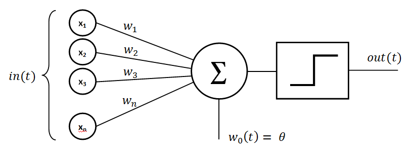
Perceptron (Source: github.com/cdipaolo)

The output of the Perceptron can be written as

and reminds of a simple linear regression with a threshold gate. While the Perceptron can be used as a building block for an universal function approximator, the singularity of the step function leads to problems when computing the gradient.

Non-linearities (Activation Functions)

Due to the singularity in the step function, other non-linear activation functions have been proposed and successfully used in NNs.

• Rectified Linear Unit (ReLU) is the most widely used non-linearity for DNNs and is computed via $y = max(0, x)$. While not being differentiable at position 0, the ReLU function greatly improves the learning process of the network due to the fact that the total gradient is simply passed to the input layer when the gate triggers.
• Leaky Rectified Linear Unit (Leaky ReLU) exploits the fact that the original ReLU is set to 0 for negative inputs and hence does not propagate a gradient for negative inputs (this is a crucial fact for initialization).
• Sigmoid non-linearities are commonly used together with regression networks in the final output layer as the outputs are bounded between $-1$ and $1$.
• Softmax non-linearities are commonly used together with classification networks in the final output layer, as the sum of the total outputs results to $1$ - similar to a probability distribution.
• Hyperbolic tangent (tanh) non-linearities are often used as a replacement for the sigmoid function leading to slightly better training results due to more stable numeric computation.

Deep Neural Networks

DL models are constructed mostly out of Convolutional (Conv) and Pooling (Pool) layers as they have been used by LeCun in the late 1980s as shown in the following figure.

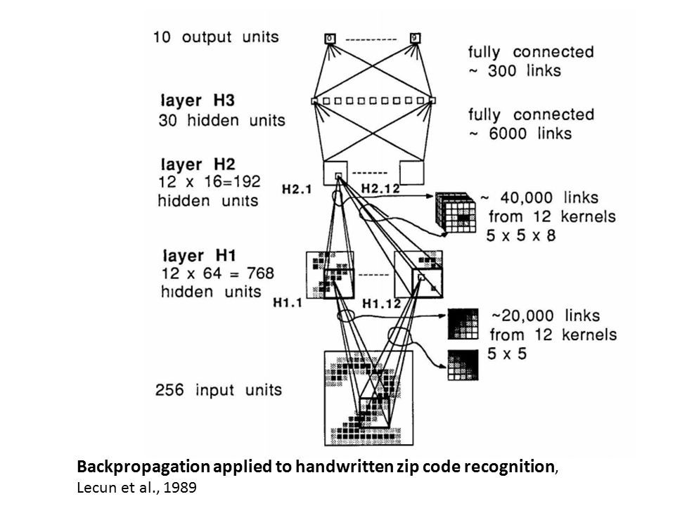
Architecture of LeNet

Convolutions

A Conv layer consists of spatial filters that are convolved along the spatial dimensions and summed up along the depth dimension of the input volume. In general one starts with a large filter size (e.g. 11x11) and a low depth (e.g. 32) and reduces the spatial filter dimensions (e.g. to 3x3) while increasing the depth (e.g. to 256) throughout the network. Due to weight sharing, they are much more efficient than fully-connected layers. A Conv layer has $w \cdot h \cdot d \cdot n_f$ number of parameters without bias ($w$ .. width of the filter, $h$ .. height of the filter, $d$ .. depth of the filter, $n_f$ number of filters) that need to be learned during training.

Pooling

Conv layers are often followed by a Pool layer in order to reduce the spatial dimension of the volume for the next filter - this is the equivalent of a subsampling operation. The pooling operation itself has no learnable parameters.

Most of the time, $max$ pooling layers are used in DL models due to the easier gradient computation. During BP, the gradient only flows in the direction of the single max activation which can be computed very efficiently. A few other architectures use $avg$ pooling, mostly at the end of a network or before the fully connected layers and without a noticeable increase in performance.

Normalization

In modern (post-sigmoid) DNNs, Normalization is necessary for stable gradients throughout the network. Due to the unbounded behavior of the ReLU activations ($y = max(0, x)$), filter responses have to be normalized. Usually this is done per batch using batch normalization or locally using a Local Response Normalization layer.

Fully Connected Layer

The FC layer works exactly as described in the previous section - it connects every output from the previous layer with each neuron. Usually, the FC layer is used at the end to combine all spatially distributed activations of the previous Conv layers. The FC layers have the highest number of parameters ($n_i \cdot n_n$, where $n_i$ is the number of outputs of the previous layer and $n_n$ is the number of neurons) in the model (almost 90%); most computing time is spent in the early Conv layers.

Final Output Layer

The final output layer of a DNN plays a crucial role for for the task of the whole network. Common choices are:

• Classification: Softmax layer, computes a value $y_{i} \in [0, 1]$ such that $\sum_i y_{i} = 1$ - can be interpreted as a probability that $x_i$ to belong to a certain class
• Regression: Sigmoid layer, predict values $y_{ij} \in [0, 1]$ for an output with $j$ dimensions.
• Regression and classification: The tasks can be combined, by connecting 2 output layers and hence outputting both values at once. This is used for object detection with a fixed number of objects, e.g. output a regression per class
• Encoder: Stop at the fully-connected layer and use it as feature space for clustering, SVM, post-processing etc.

After defining a final output layer, one need to define as well a loss function for the given task. Picking the right loss is crucial for training a DNN; common choices are:

• Classification: Cross-entropy, computes the cross-entropy between the output of the network and the ground truth label and can be used for binary and categorical outputs (via hot-one encoding)
• Regression: Squared error and mean squared error are common choices for regression problems
• Segmentation: Intersection over union is a loss function well suited for comparing overlapping regions of an image and a prediction - however, it is not well suited for DNNs because it returns 0 for non overlapping regions; MSE is a better choice

The loss function can as well be extended with a regularization term to constraint the parameters of DNN. Both L1 and L2 regularization on the filter matrices $W_i$ are commonly used.

Deep Learning Architectures

This section describes state-of-the-art DNN architectures, common parameterizations and structures in DL.

Convolutional Neural Networks (CNN)

A CNN is a neural network model that contains (multiple) convolutional layers (with a non-linear activation function) and additional pooling layers at the beginning of the network.

A convolution layer extracts image features by convolving the input with multiple filters. It contains a set of 2-dimensional filters that are stacked into a 3-dimensional volume where each filter is applied to a volume constructed from all filter responses of the previous layer. If one considers the RGB channels of a 256x256 sized input image as a 256x256x3 volume, a 5x5x3 filter would be applied along a 5x5 2-dimensional region of the image and summed up across all 3 color channels. If the first layer after the RGB volume consist of 48 filters, it is represented as a volume of 5x5x3x48 weight parameters and 48 bias parameters. Using a convolution operation on the input volume and the filter volumes, the filter response (so called activation) results in an output volume with the dimensions 251x251x48 (using stride 1 and no padding). By padding the input layer with 0s, one can force to keep the spatial dimensions of the activations constant throughout the layers.

Each convolution layer is followed by a nonlinear activation function (in DL mostly ReLU layers are used) which results in an activation with the same dimensions as the output volume of the previous convolution layer.

A pooling layer subsamples the previous layer and outputs a volume of same depth but reduced spatial dimensions. Similar to a Gaussian pyramid, pooling helps filters to activate on features in the image at a different scale. Using a max-pooling 2x2 filter with stride 2 (the filter is shifted for 2 pixels on every iteration) one ends up with a 128x128x48 volume after pooling. In general, pooling layers are used at the beginning of the network and at the end to better control the dimensions of the activations right before the fully-connected layers.

AlexNet (2012)

The following figure shows the architecture of AlexNet, the winning model for classification in the ImageNet competition in 2012. As shown in the figure, it consist of 2 parallel set of layers with both convolution and max pooling layers. The model was arranged like this due to the fact that 2 graphic cards were used in parallel for training (training AlexNet on the ImageNet dataset took 2 weeks on this setup). The filters start with a spatial dimensions 5x5 and 55 in depth (1,375 weights without bias) going to a 3x3x192 filter volume (1,728 weights without bias) towards the end of the network; hence, the filter size is decreasing but the filter depth is increasing per layer. The end of the network consists of 2 fully connected layers with 2048 nodes (4,194,304 weights without bias), and an output layer with 1000 nodes (2,048,000 weights without bias) according to the 1000 classes in the ImageNet dataset. Hence, most memory is used for the weights in the final fully connected layers; the whole model requires about 240MB in total memory. The fully connected layers at the end are needed to set the spatial filter responses in relation to each other for the resulting class prediction.

Architecture of AlexNet

The winner of the ImageNet classification task in 2013 was a tuned version of AlexNet using different initialization and optimization.

VGGNet (2014)

The VGGNet model was placed second in the ImageNet competition in 2014 by using only 3x3 filters throughout the whole network. Many different layer depths have been tested with the resulting insight that deeper is always better. This statement holds only if the deeper model can be still trained without an exploding or vanishing gradient throughout the network.

As we can see in the next figure, VGG-19 achieves very good results on the ImageNet 2012 classification dataset while having a poor accuracy vs. number of parameters ratio. To store the parameters only of VGG-19, it requires more than 500MB memory.

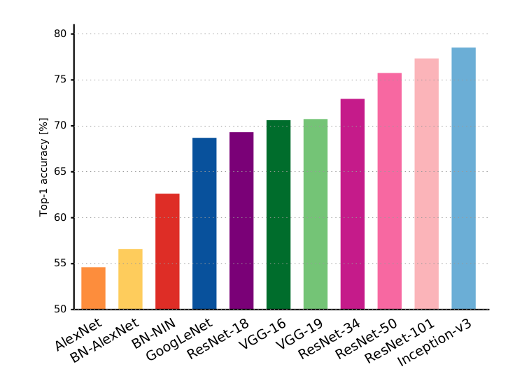
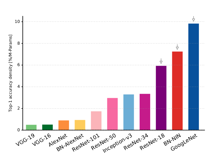
DL models Top-1 classification accuracy vs. accuracy per parameter (Source: Canziani)

GoogLeNet (2014)

The winning model in the ImageNet competition in 2014 was GoogLeNet which is even deeper than the previously discussed VGGNet. However, it uses only one tenth of the number of parameters of AlexNet due to the architecture of 9 parallel modules, the inception module. As shown in the next figure, this module uses 1x1 convolutions (so called bottleneck convolutions) to sum up the depth dimensions of the previous layers while keeping the spatial dimensions of the volume. This 1x1 convolutions allow to control/reduce the depth dimension which greatly reduces the number of used parameters due to removal of redundancy of correlated filters. It also enables to learn a set of feature across 1x1, 3x3 and 5x5 spatial dimensions in parallel mixed with a pooling of the original volume.

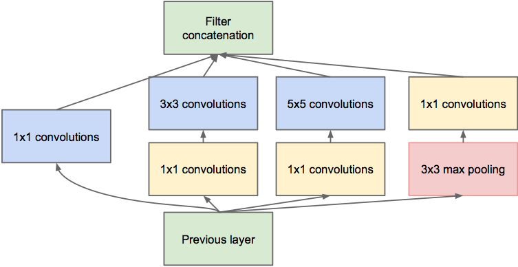
Inception module (Source COS598 (Princeton) lecture slides)

Deep Learning models 2012-2014 (Source: CaffeJS)

Deep Residual Networks (2015)

Microsoft’s residual network ResNet, the winner from ImageNet 2015 and the deepest network so far with 153 convolution layers received a top-5 classification error of 4.9% (which is slightly better than human accuracy, Source: Karpathy). By introducing residual connections (skip connections) between an input and the filter activation (as shown in the following figure), the network can learn incremental changes instead of a complete new behavior. This concept is similar to the parallel inception modules while only one filter learns the incremental changes between an input volume and its activation.

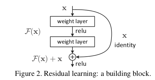Residual connections (Source: stackexchange.com)

Applications in Computer Vision

DNNs perform by a factor 10%-20% better in accuracy than methods using hand-engineered feature extraction in most computer vision tasks given enough training images and computational resources (Szegedy, Long). As shown in the next figure, the differences of DL applications in computer vision are based on the number of objects in the image and the output of the Network. This section describes in these applications and which DL approaches are commonly used.

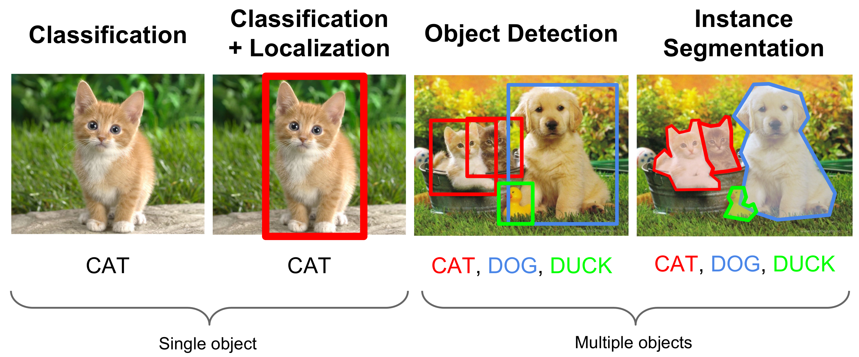Difference between Classification, Localization, Detection and Segmentation (Source: CS231n (Stanford) lecture slides)

Classification

In a classification task, a model has to predict the correct label of an image based on its contextual information which is extracted from the pixel values. Usually, one image belongs to a single class. Given an input image, the NN computes a probability value for each class; the most likely class is the resulting class for the image. An example is shown in the following figure for 8 samples from the ImageNet dataset, where the 5 most likely classes (blue bars) are displayed per input image and the correct label is shown as red bar (if it appears in these 5 classes). CNNs show a performance increase of 20% to 34% in comparison to traditional models.

DNNs for classification commonly use the “standard” architecture denoted as $IN \to [[CONV\to ReLU] \cdot N \to POOL?] \cdot M \to [FC \to ReLU] \cdot K \to FC$, where input $IN$ is a single image and output $FC$ is a fully connected layer with $m$ units (one per class). The output of each unit in the last layer corresponds to the probability that the image belongs to the class $y$. We can see that the network from 1989 had already a very similar structure (with the slight difference of using hyperbolic tangent non-linearities).

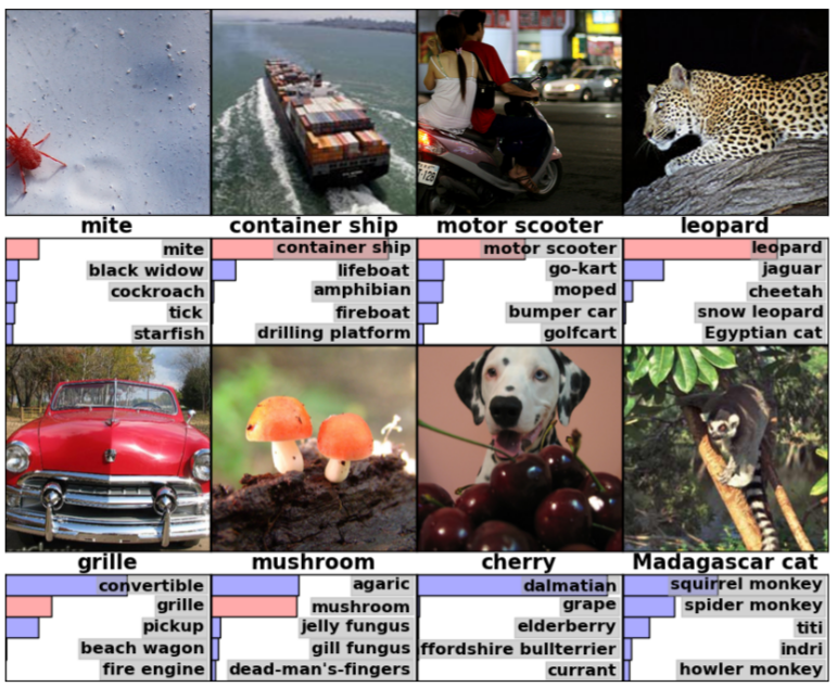Image Classification using the ImageNet dataset (Source: Krizhevsky)

Localization

In a localization task, the model needs to identify the position of an object in a sample image. Many tasks such as localization and detection can be led back to a simple binary classification task. By using a sliding window over the sample image one can determine the possibility of detecting an object at the current position of the window. After trying all possible window positions, the position of the object can be computed from the output. Due to the sliding window, the image dimensions of the input images don’t have to be fixed. Despite its simple approach, this method requires $O(n^2)$ iterations and a complex network setup and hence is not used for localization in practice.

In the simplest case with only one object in the image, the localization task can also be solved by predicting its bounding box coordinates. This is a regression problem and can be solved with a similar architecture as classification. DNNs for bounding box localization are mostly used for cropping raw input images as a preprocessing step for other applications (such as classification).

A common architecture of DNNs to solve a localization task as regression uses a fully connected layer with $4$ units (the bounding box can be identified with the coordinates of its left-top corner, width and height) in the last layer followed by a sigmoid layer. The bounding box regression can be used in combination with classification, such that bounding box coordinates can be learned for each class individually. Both methods can be combined in one DNN with one classification and one regression output.

The bounding box approach can be applied when the exact number of objects in the image is known and the image dimensions of the input images are fixed. The localization precision is bound by the rectangle geometry of the bounding box; however, also other shapes such as skewed rectangles, circles, or parallelograms can be used.

Object Detection and Image Recognition

To understand the context of images, one has to not only classify an image, but also find multiple different object instances in an image and estimate their position. This application of classifying and localizing multiple objects in an image is referred to as Object Detection. Using DNN for object detection has the advantage that it can implicitly learn complex object representations instead of manually deriving them from a kinematic model, such as a Deformable Part-based Model (DPM).

A common approach to implement object detection is a binary mask regression for each object type combined with predicting the bounding box coordinates, which results into at least 1 model per object type. This method works on both the complete image or image patches as an input, as long as the size of the input tensor is fixed. While this approach is simple a yields on average 0.15% improvement in precision compared to traditional DPMs, it requires one DNN per object type. Another difficulty are overlapping objects of the same type, as these objects are not separable in the binary mask.

The term for Image Recognition is used interchangeably for object detection, as the ability of detecting and localizing objects of different types (in an hierarchical structure) equals the ability to understand the current scene (see the following figure).

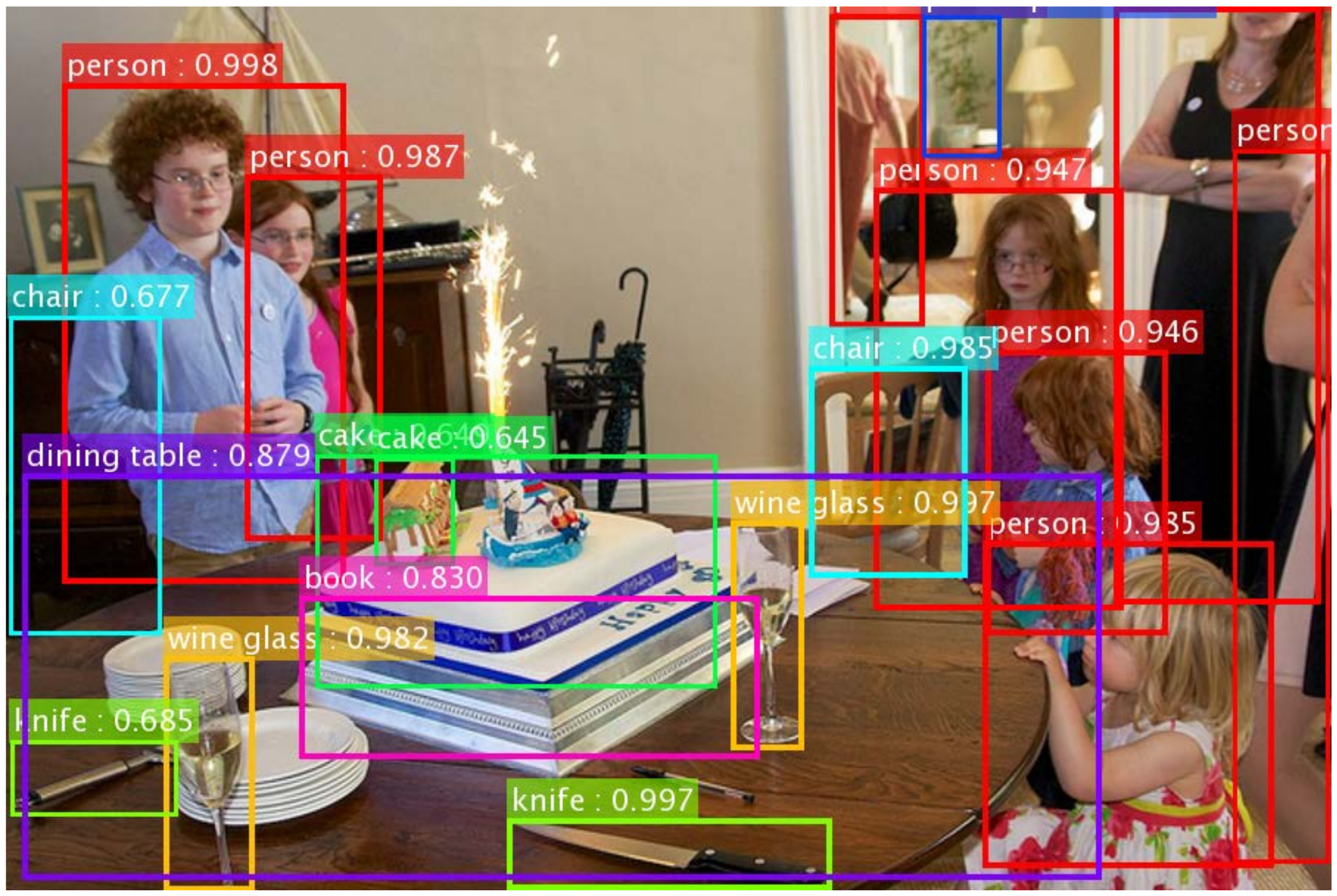Image Recognition through Object Detection (Source: He)

Segmentation

The application of Segmentation is to partition parts of an image with pixel precision, hence predicting the corresponding segment for each pixel. Thus, the network needs to predict a class value for each input pixel. convolutions and pooling both reduce the spatial dimension of the activations throughout the network which leads to the problem that the resulting activation has a smaller size than the input volume. Therefore, DNNs for segmentation need to implement an upscale strategy in order to predict per pixel.

To train a DNN for segmentation one can either input the whole image to the network and use a segmented image as ground truth (binary mask for foreground/background segmentation or pixel mask displayed in the subsequent figure) or follow a patch based approach. Using pixelwise CNNs, one can achieve up to 20% relative improvement in accuracy.

Similar to localization, segmentation can be turned into a classification problem, when using images patches of a fixed size. Instead of sliding a window over all possible locations, one can extract patches only from salient regions or distinctive segments. This approach has the advantage, that multiple patches can be stacked together as channels in the input layer to provide the network with positive and negative (or neutral) samples at the same time. This pairwise training can correct unbalanced class distributions and optimize gradient computation.

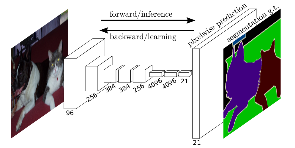Image Segmentation using a Pixel Mask (Source: Long)

As we can see in the previous figure, this upscaling process can be a gigantic fully-connected layer or an inverted DNN structure (called up-convolution or deconvolution structure).

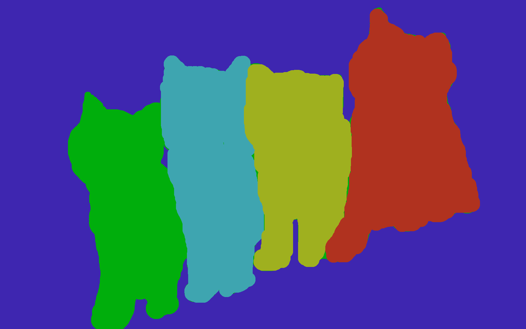Semantic vs. Instance Segmentation

The previous figure shows the 2 conceptual approaches in segmentation, the semantic segmentation (middle image) where everything from a matching class should be segmented vs. instance segmentation (right image) where every instance from a class should be segmented.

In semantic segmentation, multi-scale architecture are used that upsample outputs and combine the results with traditional bottom-up segmentations. In a different approach, the complete upscaling process can learned via an inverted DNN structure. By adding skip connections from lower layers to higher upsampled levels one can also learn incremental structures and perform local refinement on the downsampled image.

Instance segmentation is often referred to as simultaneous detection and segmentation and is a very challenging task. Most commonly window functions are used for applying classification and segmentation on all possible sets of input patches. This requires unnecessary computational resources for regions that don’t contain any objects. Hence, so called region proposals techniques have been introduced, to optimize the selection of regions that can be further selected as a patch input for the segmentation. Fast R-CNN is a method using the ResNet architecture and implements a pipelines similar to object detection.

Image Encoding

A very common task of DNNs is image encoding, hence transforming and image from its original representation to a lower dimensional feature space. This task is often performed implicitly due to the fact that the last fully-connected layer of each DNN learns this encoding automatically while trained on a specific supervised task. At the end of the training, the last fully-connected layer contains a fixed-sized low-dimensional numeric representation of the input image that can be used as an input for conventional machine learning approaches such as SVM, linear regression, etc.

Using up-convolutional structures, one can also implement unsupervised auto-encoding networks. However, due to the implicit learning through classification and the high computational complexity of up-convolutional networks this is mostly done by training on a supervised method such as classification.

Summary

Using the correct DNN architecture for an application of DL in computer vision requires knowledge of the specific problem and limitations, such as fixed number of objects in localization and fixed image dimensions in pixelwise segmentation. However, DL architectures always perform better than classical hand-engineered approaches with a factor 10% to 20% in accuracy given enough training samples and computing power. However, in many DL applications such as detection and recognition, more than one model is required to predict all possible object types. Hence, training multiple models requires linear costs for training time and computation.

Resources

• CS231n (Stanford) Video Lectures
• CS231n (Stanford) Lecture Notes
• Going Deeper with Convolutions
• Rethinking the Inception Architecture for Computer Vision
• Slides from my talk at the University

References

• F. Rosenblatt, “The perceptron, a perceiving and recognizing automaton Project Para”, in Cornell Aeronautical Laboratory, 1957.

• P. Werbos, “Beyond Regression: New Tools for Prediction and Analysis in the Behavioral Sciences”, in PhD thesis, Harvard University, Cambridge, 1974.

• D. E. Rumelhart, G. E. Hinton, and R. J. Williams, “Learning representations by back-propagating errors”, in Nature, vol. 323, pp. 533-536, 1986.

• Y. LeCun, B. Boser, J. S. Denker, D. Henderson, R. E. Howard, W. Hubbard, and L. D. Jackel, “Handwritten digit recognition with a back-propagation network”, in Advances in Neural Information Processing Systems (NIPS 1989), D. Touretzky (Ed.), vol. 2, pp. 533-536, 1990.

• J. Schmidhuber, “Deep Learning in Neural Networks: An Overview”, in CoRR, 2014.

• I. Goodfellow, Y. Bengio and A. Courville, “Deep Learning”, in preparation for MIT Press, 2016.

• X. Glorot and Y. Bengio, “Understanding the difficulty of training deep feedforward neural networks”, in Proceedings of the International Conference on Artificial Intelligence and Statistics, 2010.

• K. He, X. Zhang, S. Ren and J. Sun, “Deep Residual Learning for Image Recognition”, CoRR, 2015.

• K. He, X. Zhang, S. Ren and J. Sun, “Delving Deep into Rectifiers: Surpassing Human-Level Performance on ImageNet Classification”, CoRR, 2015.

• A. Krizhevsky, I. Sutskever and G. Hinton, “ImageNet Classification with Deep Convolutional Neural Networks”, in Advances in Neural Information Processing Systems, 2012.

• A. Radford, L. Metz and S. Chintala, “Unsupervised Representation Learning with Deep Convolutional Generative Adversarial Networks”, CoRR, 2015.

• E. Smirnov, D. Timoshenko and S. Andrianov, “Comparison of Regularization Methods for ImageNet Classification with Deep Convolutional Neural Networks”, in AASRI Procedia, vol. 6, pp. 89-94, 2014.

• C. Szegedy, W. Liu, Y. Jia, P. Sermanet, S. Reed, D. Anguelov, D. Erhan, V. Vanhoucke and A. Rabinovich, “Going Deeper with Convolutions”, CoRR, 2014.

• M. Zeiler and R. Fergus, “Visualizing and Understanding Convolutional Networks”, in COMPUTER VISION – ECCV 2014, 1st ed., D. Fleet, T. Pajdla, B. Schiele and T. Tuytelaars, Ed. 2014.

• S. Zhou, Q. Chen and X. Wang, “Convolutional Deep Networks for Visual Data Classification”, in Neural Process Letters, vol. 38, no. 1, pp. 17-27, 2012.

• D.P. Kingma and J. Ba, “Adam: A Method for Stochastic Optimization”, in The International Conference on Learning Representations (ICLR), 2015.

• M. Henaff, A. Szlam, and Y. LeCun, “Orthogonal RNNs and Long-Memory Tasks”, CoRR, 2016.

• C. Szegedy, A. Toshev, and D. Erhan, “Deep Neural Networks for Object Detection”, in Advances in Neural Information Processing Systems 26, C. Burges (Ed.), pp. 2553-2561, 2013.

• K. Simonyan and A. Zisserman, “Very Deep Convolutional Networks for Large-Scale Image Recognition”, CoRR, 2014.

• P. Sermanet, D. Eigen, X. Zhang, M. Mathieu, R. Fergus, and Y. LeCun, “Overfeat: Integrated recognition, localization and detection using convolutional networks”, in ICLR, 2014.

• J. Long, E. Shelhamer, and T. Darrell, “Fully Convolutional Networks for Semantic Segmentation”, CoRR, 2014.

• M. Lin, Q. Chen and S. Yan, “Network In Network”, CoRR, 2013.

• S. Ioffe and C. Szegedy, “Batch Normalization: Accelerating Deep Network Training by Reducing Internal Covariate Shift”, CoRR, 2015.

• N. Srivastava, G. Hinton, A. Krizhevsky, I. Sutskever and R. Salakhutdinov, “Dropout: A Simple Way to Prevent Neural Networks from Overfitting”, in Journal of Machine Learning Research, vol. 15, pp. 1929-1958, 2014.

• F. Li, A. Karpathy, and J. Johnson, “Spatial Localization and Detection”, in CS231n: Convolutional Neural Networks for Visual Recognition, lecture slides, p. 8, 2016.

• D. Ciregan, U. Meier, and J. Schmidhuber, “Multi-column deep neural networks for image classification”, in IEEE Conference on Computer Vision and Pattern Recognition (CVPR), 2012 pp. 3642-3649, 2012.

• C. Farabet, C. Couprie, L. Najman, and Y. LeCun, “Learning Hierarchical Features for Scene Labeling”, in IEEE Transactions on Pattern Analysis and Machine Intelligence, vol. 35, no. 8, pp. 1915-1929, 2013.

• H. Noh, S. Hong, and B. Han, “Learning Deconvolution Network for Semantic Segmentation”, CoRR, 2015.

• B. Hariharan, P. Arbeláez, R. Girshick, and J. Malik, “Simultaneous Detection and Segmentation”, in European Conference on Computer Vision (ECCV), 2014.

• J. Dai, K. He, and J. Sun, “Instance-aware Semantic Segmentation via Multi-task Network Cascades”, CoRR, 2015.

• A.M. Saxe, J.L. McClelland and S. Ganguli, “Exact solutions to the nonlinear dynamics of learning in deep linear neural networks”, CoRR, 2015.

• T. Tieleman and G. Hinton, “RMSprop Gradient Optimization”, in Neural Networks for Machine Learningn, lecture slides, p. 29, 2014.

• A. Canziani, A. Paszke and E. Culurciello, “An Analysis of Deep Neural Network Models for Practical Applications”, CoRR, 2016.